Creating Formulas in Excel 2010
Formulas in MS Excel
Formulas are the Bread and butter of worksheet. Without formula, worksheet will be just simple tabular representation of data. A formula consists of special code, which is entered into a cell. It performs some calculations and returns a result, which is displayed in the cell.
Formulas use a variety of operators and worksheet functions to work with values and text. The values and text used in formulas can be located in other cells, which makes changing data easy and gives worksheets their dynamic nature. For example, you can quickly change the data in a worksheet and formulas works.
Elements of Formulas
A formula can consist of any of these elements −
- Mathematical operators, such as +(for addition) and *(for multiplication)Example −
- =A1+A2 Adds the values in cells A1 and A2.
- Values or textExample −
- =200*0.5 Multiplies 200 times 0.15. This formula uses only values, and it always returns the same result as 100.
- Cell references (including named cells and ranges)Example −
- =A1=C12 Compares cell A1 with cell C12. If the cells are identical, the formula returns TRUE; otherwise, it returns FALSE.
- Worksheet functions (such as SUMor AVERAGE)Example −
- =SUM(A1:A12) Adds the values in the range A1:A12.
Creating Formula
For creating a formula you need to type in the Formula Bar. Formula begins with '=' sign. When building formulas manually, you can either type in the cell addresses or you can point to them in the worksheet. Using the Pointing method to supply the cell addresses for formulas is often easier and more powerful method of formula building. When you are using built-in functions, you click the cell or drag through the cell range that you want to use when defining the function’s arguments in the Function Arguments dialog box. See the below screen shot.
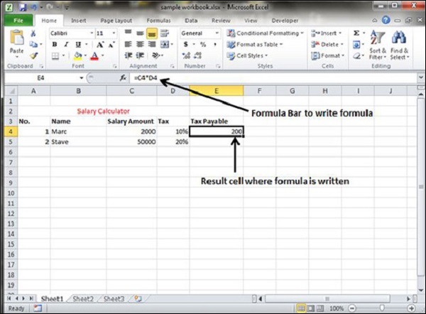
As soon as you complete a formula entry, Excel calculates the result, which is then displayed inside the cell within the worksheet (the contents of the formula, however, continue to be visible on the Formula bar anytime the cell is active). If you make an error in the formula that prevents Excel from being able to calculate the formula at all, Excel displays an Alert dialog box suggesting how to fix the problem.
Copying Formulas in Excel 2010
Copying Formulas in MS Excel
Copying formulas is one of the most common tasks that you do in a typical spreadsheet that relies primarily on formulas. When a formula uses cell references rather than constant values, Excel makes the task of copying an original formula to every place that requires a similar formula.
Relative Cell Addresses
MS Excel does it automatically adjusting the cell references in the original formula to suit the position of the copies that you make. It does this through a system known as relative cell addresses, where by the column references in the cell address in the formula change to suit their new column position and the row references change to suit their new row position.
Let us see this with the help of example. Suppose we want the sum of all the rows at last, then we will write a formula for first column i.e. B. We want sum of the rows from 3 to 8 in the 9th row.
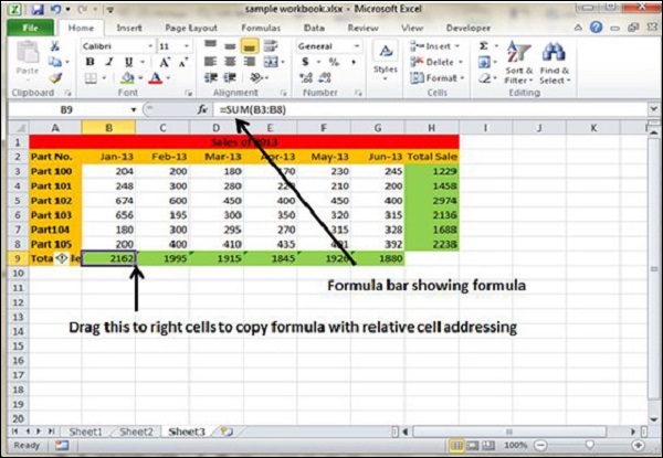
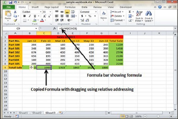
After writing formula in the 9th row, we can drag it to remaining columns and the formula gets copied. After dragging we can see the formula in the remaining columns as below.
- column C : =SUM(C3:C8)
- column D : =SUM(D3:D8)
- column E : =SUM(E3:E8)
- column F : =SUM(F3:F8)
- column G : =SUM(G3:G8)
Formula Reference in Excel 2010
Cell References in Formulas
Most formulas you create include references to cells or ranges. These references enable your formulas to work dynamically with the data contained in those cells or ranges. For example, if your formula refers to cell C2 and you change the value contained in C2, the formula result reflects new value automatically. If you didn’t use references in your formulas, you would need to edit the formulas themselves in order to change the values used in the formulas.
When you use a cell (or range) reference in a formula, you can use three types of references − relative, absolute, and mixed references.
Relative Cell References
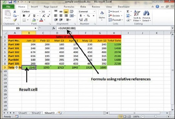
The row and column references can change when you copy the formula to another cell because the references are actually offsets from the current row and column. By default, Excel creates relative cell references in formulas.
Absolute Cell References
The row and column references do not change when you copy the formula because the reference is to an actual cell address. An absolute reference uses two dollar signs in its address: one for the column letter and one for the row number (for example, $A$5).
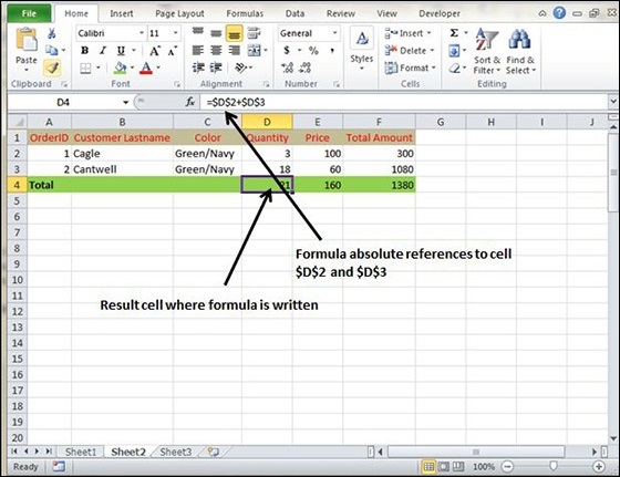
Mixed Cell References
Both the row or column reference is relative and the other is absolute. Only one of the address parts is absolute (for example, $A5 or A$5).
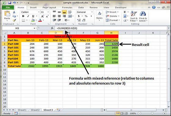
Using Functions in Excel 2010
Functions in Formula
Many formulas you create use available worksheet functions. These functions enable you to greatly enhance the power of your formulas and perform calculations that are difficult if you use only the operators. For example, you can use the LOG or SIN function to calculate the Logarithm or Sin ratio. You can’t do this complicated calculation by using the mathematical operators alone.
Using Functions
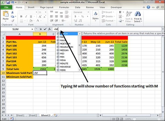
When you type = sign and then type any alphabet you will see the searched functions as below.
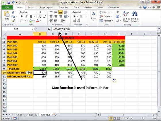
Suppose you need to determine the largest value in a range. A formula can’t tell you the answer without using a function. We will use formula that uses the MAX function to return the largest value in the range B3:B8 as =MAX(A1:D100).
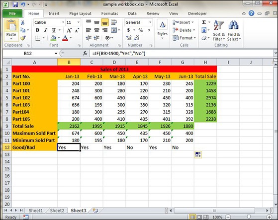
Another example of functions. Suppose you want to find if the cell of month is greater than 1900 then we can give Bonus to Sales representative. The we can achieve it with writing formula with IF functions as =IF(B9>1900,"Yes","No")
Function Arguments
In the above examples, you may have noticed that all the functions used parentheses. The information inside the parentheses is the list of arguments.
Functions vary in how they use arguments. Depending on what it has to do, a function may use.
- No arguments − Examples − Now(), Date(), etc.
- One argument − UPPER(), LOWER(), etc.
- A fixed number of arguments − IF(), MAX(), MIN(), AVERGAGE(), etc.
- Infinite number of arguments
- Optional arguments
Built-in Functions in Excel 2010
Built In Functions
MS Excel has many built in functions, which we can use in our formula. To see all the functions by category, choose Formulas Tab » Insert Function. Then Insert function Dialog appears from which we can choose the function.
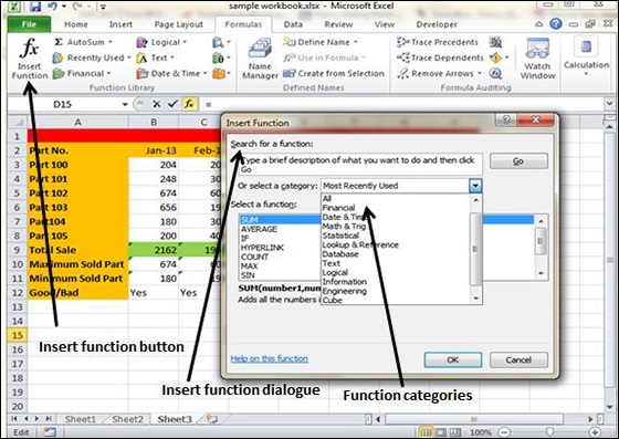
Functions by Categories
Let us see some of the built in functions in MS Excel.
- Text Functions
- LOWER − Converts all characters in a supplied text string to lower case
- UPPER − Converts all characters in a supplied text string to upper case
- TRIM − Removes duplicate spaces, and spaces at the start and end of a text string
- CONCATENATE − Joins together two or more text strings.
- LEFT − Returns a specified number of characters from the start of a supplied text string.
- MID − Returns a specified number of characters from the middle of a supplied text string
- RIGHT − Returns a specified number of characters from the end of a supplied text string.
- LEN − Returns the length of a supplied text string
- FIND − Returns the position of a supplied character or text string from within a supplied text string (case-sensitive).
- Date & Time
- DATE − Returns a date, from a user-supplied year, month and day.
- TIME − Returns a time, from a user-supplied hour, minute and second.
- DATEVALUE − Converts a text string showing a date, to an integer that represents the date in Excel's date-time code.
- TIMEVALUE − Converts a text string showing a time, to a decimal that represents the time in Excel.
- NOW − Returns the current date & time.
- TODAY − Returns today's date.
- Statistical
- MAX − Returns the largest value from a list of supplied numbers.
- MIN − Returns the smallest value from a list of supplied numbers.
- AVERAGE − Returns the Average of a list of supplied numbers.
- COUNT − Returns the number of numerical values in a supplied set of cells or values.
- COUNTIF − Returns the number of cells (of a supplied range), that satisfies a given criteria.
- SUM − Returns the sum of a supplied list of numbers
- Logical
- AND − Tests a number of user-defined conditions and returns TRUE if ALL of the conditions evaluate to TRUE, or FALSE otherwise
- OR − Tests a number of user-defined conditions and returns TRUE if ANY of the conditions evaluate to TRUE, or FALSE otherwise.
- NOT − Returns a logical value that is the opposite of a user supplied logical value or expression i.e. returns FALSE if the supplied argument is TRUE and returns TRUE if the supplied argument is FAL
- Math & Trig
- ABS − Returns the absolute value (i.e. the modulus) of a supplied number.
- SIGN − Returns the sign (+1, -1 or 0) of a supplied number.
- SQRT − Returns the positive square root of a given number.
- MOD − Returns the remainder from a division between two supplied numbers.
No comments:
Post a Comment